欢迎来到DeepModeling教程!

大家好，这里是DeepModeling项目的教程。

使用DeePMD-Kit

本教程告诉你如何使用DeePMD-kit，详细的信息，你可以查看 [DeePMD-kit文档](https://docs.deepmodeling.org/projects/deepmd/en/latest/)。

简介

在过去的几十年时间里，因为在凝聚态物理、材料科学、高分子化学和分子生物学等领域的广泛应用，分子动力学模拟方法被越来越多人关注和使用，这种模拟手段让研究人员有能力去观察原子或分子间的运动行为，在一些实验手段极难，甚至无法探索的问题上，分子动力学模拟方法能够极大地拓宽我们的认知边界。

众所周知，分子动力学模拟的结果好坏取决于势函数的准确性，如何能精确地表示势函数是分子动力学模拟中极其重要的问题。经验势模型与量子力学模型是最为常用的两种方法，经验势通常由物理直觉出发，给出关于体系能量的数项组成，因为形式简单而通常有较快的计算速度，但是无法保证精度。与之相反，量子力学模型通过近似求解电子结构来计算原子的受力和能量，具有非常高的精度，但随之而来的是计算速度的限制，无法应用于更大型或更长时间的计算中。总而言之，在如何精确地表示势能面这个问题上，人们需要在精度和速度上做出选择，无法两者兼顾。

但随着AI for Science浪潮的到来，机器学习势函数正在帮助人们跨越精度与速度之间的鸿沟。描述子与机器学习算法是机器学习势函数的两个主要组成部分。描述子用于保证所研究结构的对称性，机器学习算法通过训练量子力学精度下的数据，建立原子结构与体系能量之间的函数关系，训练完成后，机器学习势函数能给出与训练数据相同的量子力学精度，如果训练数据是由密度泛函理论计算得出，那么机器学习势函数也会是密度泛函理论的精度，但与密度泛函理论的计算量随着研究体系扩大而三次方增长不同，机器学习势函数的计算量只与体系大小呈线性关系。

到目前为止，已经有相当多的研究提出了不同形式的机器学习势函数模型，例如Behler-Parrinello neural network potentials(BPNNP)[1], Gaussian approximation potentials(GAP)[2], spectral neighbor analysis potentials(SNAP)[3], ANI-1[4], SchNet[5] and Deep Potential[[6],[7],[8]],虽然已取得了较大成功，但机器学习势函数模型仍有很多极具挑战性的问题等待解决[9],例如忽略截断半径外的相互作用导致的系统性预测误差[10]等问题

本章节将重点介绍DP模型，除了能达到量子力学的精度外，目前的DP模型还具有以下特点：(1)易于保持体系的对称性，尤其是当体系存在多种元素时；(2)计算效率高，比密度泛函理论至少快五个数量级；(3)端到端模型，减少人为干预的可能；(4)支持MPI和GPU，能够在现代异构高性能超级计算机上高效运行。目前，DP模型已经成功地应用在水和含水系统[[11],[12],[13],[14]],金属和合金[[15],[16],[17],[18]],相图[[19],[20],[21]],高熵陶瓷[[22],[23]],化学反应[[24],[25],[26]],固态电解质[27],离子液体[28]等研究领域中。对于最近DP模型在材料领域方面的研究，我们参考了此篇文献[29].

简易安装

DeePMD-kit有很多简单的的安装方式，你可以按需选择。如果你希望独立编译，可以跳转到下一部分。

完成了安装流程后，文件中会自带两个已经编译好的程序：DeePMD-kit(dp)和LAMMPS(lmp)，你可以尝试输入dp -h和lmp -h来获取帮助信息，考虑到你会选择并行地训练模型和运行LAMMPS，mpirun同样已编译好并可供使用。

安装离线软件包

CPU和GPU版本的离线软件包都在可以the Releases page中找到

由于Github对文件大小的限制，一些安装包被拆分成两个文件，我们可以将拆分文件都下载下来再进行合并。

cat deepmd-kit-2.0.0-cuda11.3_gpu-Linux-x86_64.sh.0 deepmd-kit-2.0.0-cuda11.3_gpu-Linux-x86_64.sh.1 > 
deepmd-kit-2.0.0-cuda11.3_gpu-Linux-x86_64.sh

利用Conda安装

DeePMD-kit可以利用Conda安装，不过首先需要安装好Anaconda或者Miniconda

安装好Anaconda或Miniconda之后，我们可以创建一个包含CPU版本的DeePMD-kit和LAMMPS的虚拟环境

conda create -n deepmd deepmd-kit=*=*cpu libdeepmd=*=*cpu lammps-dp -c https://conda.deepmodeling.org

同理，也可以创建包含GPU版本的虚拟环境

conda create -n deepmd deepmd-kit=*=*gpu libdeepmd=*=*gpu lammps-dp cudatoolkit=11.3 horovod -c https://conda.deepmodeling.org

CUDA Toolkit版本可以按需从10.1或11.3中选择

如果你想安装指定版本的DeePMD-kit，例如2.0.0：

conda create -n deepmd deepmd-kit=2.0.0=*cpu libdeepmd=2.0.0=*cpu lammps-dp=2.0.0 horovod -c https://conda.deepmodeling.org

创建虚拟环境后，每次使用前需要激活环境：

conda activate deepmd

利用docker安装

DeePMD-kit同样可以通过docker安装

获取CPU版本：

docker pull ghcr.io/deepmodeling/deepmd-kit:2.0.0_cpu

获取GPU版本：

docker pull ghcr.io/deepmodeling/deepmd-kit:2.0.0_cuda10.1_gpu

获取ROCm版本：

docker pull deepmodeling/dpmdkit-rocm:dp2.0.3-rocm4.5.2-tf2.6-lmp29Sep2021

如果你想从源码开始安装DeePMD-kit，请点此处

理论

在介绍DP具体方法之前, 我们先介绍一些定义。首先我们可以对一个包含 $N$ 个原子的系统定义一个坐标矩阵 $\mathcal{R} \in \mathbb{R}^{N \times 3}$ ，

$\mathcal{R}=\left\{{r}_{1}^{T}, \cdots, {r}_{i}^{T}, \cdots, {r}_{N}^{T}\right\}^{T}, {r}_{i}=\left(x_{i}, y_{i}, z_{i}\right),(1)$

${r}_{i}$ 表示原子 $i$ 的三维笛卡尔坐标。为了之后DP理论介绍的方便，我们可以将坐标矩阵 $\mathcal{R}$ 转换成一系列局域坐标矩阵 $\left\{{\mathcal{R}}^{i}\right\}_{i=1}^{N}$ ,

${\mathcal{R}}^{i}=\left\{{r}_{1 i}^{T}, \cdots, {r}_{j i}^{T}, \cdots, {r}_{N_{i}, i}^{T}\right\}^{T}, {r}_{j i}=\left(x_{j i}, y_{j i}, z_{j i}\right),(2)$

其中 $N_{i}$ 是原子 $i$ 在截断半径为 $r_{c}$ 下的近邻原子数， $j \left(1 \leq j \leq N_{i}\right)$ 表示原子 $i$ 的近邻原子编号, ${r}_{j i} \equiv {r}_{j}-{r}_{i}$ 表示的是原子 $j$ 和原子 $i$ 之间的相对距离。

在DP方法中, 一个系统的总能量 $E$ 可以被看作是各个原子的局域能量贡献的总和

$E=\sum_{i} E_{i},(3)$

其中 $E_{i}$ 是原子 $i$ 的局域能量. $E_{i}$ 取决于原子 $i$ 的局域环境:

$E=\sum_{i} E_{i}=\sum_{i} E\left(\mathcal{R}^{i}\right),(4)$

从 ${\mathcal{R}}^{i}$ 到 $E_{i}$ 的映射可以由两步来构建。第一步，如同 figure 里展示的一样, ${\mathcal{R}}^{i}$ 要映射到特征矩阵，或者说描述子 ${\mathcal{D}}^{i}$ ，这里的 ${\mathcal{D}}^{i}$ 保留了体系的平移、旋转和置换不变性。具体来说， ${\mathcal{R}}^{i} \in \mathbb{R}^{N_{i} \times 3}$ 首先被映射到一个扩展矩阵 $\tilde{{\mathcal{R}}}^{i} \in \mathbb{R}^{N_{i} \times 4}$ ，

$\left\{x_{j i}, y_{j i}, z_{j i}\right\} \mapsto\left\{s\left(r_{j i}\right), \hat{x}_{j i}, \hat{y}_{j i}, \hat{z}_{j i}\right\},(5)$

其中 $\hat{x}_{j i}=\frac{s\left(r_{j i}\right) x_{j i}}{r_{j i}}$ , $\hat{y}_{j i}=\frac{s\left(r_{j i}\right) y_{j i}}{r_{j i}}$ , $\hat{z}_{j i}=\frac{s\left(r_{j i}\right) z_{j i}}{r_{j i}}$ . $s\left(r_{j i}\right)$ 是一个权重函数，用来减少离原子 $i$ 比较远的原子的权重, 定义如下:

$s\left(r_{j i}\right)= \begin{cases}\frac{1}{r_{j i}}, & r_{j i}<r_{c s} \\ \frac{1}{r_{j i}} \{ {(\frac{r_{j i} - r_{c s}}{ r_c - r_{c s}})}^3 (-6 {(\frac{r_{j i} - r_{c s}}{ r_c - r_{c s}})}^2 +15 \frac{r_{j i} - r_{c s}}{ r_c - r_{c s}} -10) +1 \}, & r_{c s}<r_{j i}<r_{c} \\ 0, & r_{j i}>r_{c}\end{cases},(6)$

其中 $r_{j i}$ 是原子 $i$ 和原子 $j$ 之间的欧式距离, $r_{cs}$ 是“平滑截断半径”。引入 $s\left(r_{j i}\right)$ 之后 $\tilde{{\mathcal{R}}}^{i}$ 里的成分会从 $r_{cs}$ 到 $r_{c}$ 平滑地趋于零。接着 $\{s\left(r_{j i}\right)\}_{j=1}^{N_i}$ , i.e. 也就是 $\tilde{{\mathcal{R}}}^{i}$ 的第一列, 被一个嵌入神经网络映射到一个嵌入矩阵 $\mathcal{G}^{i 1} \in \mathbb{R}^{N_{i} \times M_{1}}$ . 选取 ${\mathcal{G}}^{i 1} \in \mathbb{R}^{N_{i} \times M_{1}}$ 的前 $M_{2}(<M_{1})$ 列，我们就得到了另外一个嵌入矩阵 $\mathcal{G}^{i 2} \in \mathbb{R}^{N_{i} \times M_{2}}$ . 最后，我们就可以得到原子 $i$ 的描述子 ${\mathcal{D}}^{i}$ ：

$\mathcal{D}^{i}=\left(\mathcal{G}^{i 1}\right)^{T} \tilde{\mathcal{R}}^{i}\left(\tilde{\mathcal{R}}^{i}\right)^{T} \mathcal{G}^{i 2},(7)$

在描述子中, 平移和旋转不变性是由矩阵乘积 $\tilde{\mathcal{R}}^{i}\left(\tilde{\mathcal{R}}^{i}\right)^{T}$ 来保证的, 置换不变性是由矩阵乘积 $\left(\mathcal{G}^{i}\right)^{T} \tilde{\mathcal{R}}^{i}$ 来保证的。

第二步, 每一个描述子 ${\mathcal{D}}^{i}$ 都由一个拟合神经网络被映射到一个局域的能量 $E_{i}$ 上面。

嵌入神经网络 $\mathcal{N}^e$ 和拟合神经网络 $\mathcal{N}^f$ 都是包含很多隐藏层的前馈神经网络。前一层的数据 $d_{l}^{\mathrm{in}}$ 是由一个线性运算和一个非线性的激活函数传递到下一层的数据 $d_{k}^{\mathrm{out}}$ .

$d_{k}^{o u t}=\varphi\left(\sum_{k l} w_{k l} d_{l}^{i n}+ b_{k}\right),(8)$

在公式（8）中, ${w}_{k l}$ 是权重参数, ${b}_{k}$ 是偏置参数， $\varphi$ 是一个非线性的激活函数. 需要注意的是在最后一层的输出节点是没有非线性激活函数的。在嵌入网络和拟合网络中的参数由最小化代价函数 $L$ 得到:

$L\left(p_{\epsilon}, p_{f}, p_{\xi}\right)=\frac{p_{\epsilon}}{N} \Delta \epsilon^{2}+\frac{p_{f}}{3 N} \sum_{i}\left|\Delta {F}_{i}\right|^{2}+\frac{p_{\xi}}{9N}\|\Delta \xi\|^{2},(9)$

其中 $\Delta \epsilon$ , $\Delta {F}_{i}$ , 和 $\Delta \xi$ 分别表示能量、力和维里的方均根误差 (RMSE) . 在训练的过程中, 前置因子 $p_{\epsilon}$ , $p_{f}$ , 和 $p_{\xi}$ 由公式

$p(t)=p^{\operatorname{limit}}\left[1-\frac{r_{l}(t)}{r_{l}^{0}}\right]+p^{\operatorname{start}}\left[\frac{r_{l}(t)}{r_{l}^{0}}\right],(10)$

来决定，其中 $r_{l}(t)$ 和 $r_{l}^{0}$ 分别表示在训练步骤 $t$ 和训练步骤0 时的误差。 $r_{l}(t)$ 的定义为

$r_{l}(t)=r_{l}^{0} \times d_{r}^{t / d_{s}},(11)$

其中 $d_{r}$ 和 $d_{s}$ 分别表示的是学习衰减率以及衰减步骤。学习衰减率 $d_{r}$ 要严格小于1。读者如果想要了解更多细节，可以查看 DeepPot-SE (DP)方法的原始文章DeepPot-SE.

如何在五分钟之内Setup一次DeepMD-kit训练

DeepMD-kit 是一款实现深度势能(Deep Potential)的软件。虽然网上已经有很多关于DeepMD-kit的资料和信息以及官方指导文档，但是对于小白用户仍不是很友好。今天，这篇教程将在五分钟内带你入门DeepMD-kit。

首先让我们先关注一下DeepMD-kit的训练流程：

数据准备->训练->冻结/压缩模型

是不是觉得很简单？让我们对这几个步骤作更深的阐述：

数据准备 : 将DFT的计算结果转化成DeepMD-kit能够识别的数据格式。
训练 : 使用前一步准备好的数据通过DeepMD-kit来训练一个深度势能模型(Deep Potential Model)
冻结/压缩模型 :最后我们需要做的就是冻结/压缩一个训练过程中输出的重启动文件来生成模型。相信你已经迫不及待想要上手试试啦！让我们开始吧！

##1.4.1. 下载教程中提供的数据第一步，让我们下载和解压教程中提供给我们的数据:

 $ wget https://github.com/likefallwind/DPExample/raw/main/DeePMD-kit-FastLearn.tar
 $ tar xvf DeePMD-kit-FastLearn.tar

如果因为网络问题连不上github，你可以通过如下代码下载 :

 $ wget https://gitee.com/likefallwind/dpexamples/raw/main/DeePMD-kit-FastLearn.tar
 $ tar xvf DeePMD-kit-FastLearn.tar

然后我们可以进入到下载好的数据目录检查一下 :

$ cd DeePMD-kit-FastLearn
$ ls
00.data 01.train data

##1.4.2. 数据准备现在让我们进入到00.data目录 :

$ cd 00.data
$ ls
OUTCAR

目录当中有一个VASP计算结果输出OUTCAR文件，我们需要将他转换成DeepMD-kit数据格式。DeepMD-kit数据格式在官方文档中有相应的介绍，但是看起来很复杂。别怕，这里将介绍一款数据转换神奇dpdata，只用一行python命令就能处理好数据，是不是超级方便！

import dpdata
dpdata.LabeledSystem('OUTCAR').to('deepmd/npy', 'data', set_size=200)

在上面的命令中，我们将VASP计算结果输出文件OUTCAR转换成DeepMD-kit数据格式并保存在data目录当中，其中npy是指numpy压缩格式，也就是DeepMD-kit训练所用的数据格式。

假设你已经有了分子动力学输出“OUTCAR”文件，其中包含了1000帧。set_size=200将会将1000帧分成五个子集，每份200帧，分别命名为data/set.000~data/set.004。这五个子集中，data/set.000~data/set.003将会被DeepMD-kit用作训练集，data/set.004将会被用作测试集。如果设置set_size=1000，那么只有一个集合，这个集合既是训练集又是测试集(当然这个测试的参考意义就不大了)。

教程当中提供的OUTCAR只包含了一帧数据，所以在data目录(与OUTCAR在同一目录)当中将只会出现一个集合data/set.000。如果你想用对数据做一些其他的处理，更详细的信息请参考下一章。

我们将跳过更详细的处理步骤，接下来我们进入到根目录当中使用教程已经为你提供好的数据。

$ cd ..
$ ls
00.data 01.train data

##1.4.3. Training 开始DeepMD-kit训练需要准备一个输入脚本，大家是不是还有没从被INCAR脚本支配的恐惧中走出来？别怕，配置DeepMD-kit比配置VASP简单多了。我们已经为你准备好了input.json，你可以在”01.train”目录当中找到它

$ cd 01.train
$ ls
input.json

DeepMD-kit的强大之处在于一样的训练参数可以适配不同的系统，所以我们只需要微调input.json来开始训练。首先需要修改的参数是 :

 "type_map":     ["O", "H"],

DeepMD-kit中对每个原子类型是按从0开始的整数编号的。这个参数给了这样的编号系统中每个原子类型一个元素名。这里我们照抄data/type_map.raw的内容就好。比如我们改成 :

"type_map":    ["A", "B","C"],

其次，我们修改一下邻居搜索参数 :

"sel":       [46, 92],

这个list中每个数给出了某原子的邻居中，各个类型的原子的最大数目。比如46就是类型为0,元素为O的邻居最多有46个。这里我们换成了ABC，这个参数我们要相应的修改。不知道最大邻居数怎么办？可以用体系的密度粗略估计一个。或者可以盲试一个数，如果不够大DeepMD-kit会告诉你的。下面我们改成了 :

"sel":       [64, 64, 64]

此外我们需要修改的参数是"training_data"中的"systems"

"training_data":{
      "systems":     ["../data/data_0/", "../data/data_1/", "../data/data_2/"],

以及"validation_data"

 "validation_data":{
      "systems":     ["../data/data_3"],

这里我将稍微介绍一下data system的定义。DeepMD-kit认为，具有同样原子数，且原子类型相同的数据能够形成一个system。我们的数据是从一个分子动力学模拟生成的，当然满足这个条件，因此可以放到一个system中。dpdata也是这么帮我们做的。当数据无法放到一个system中时，就需要设multiple systems，写成一个list。

 "systems": ["system1", "system2"]

最后我们还需要改另外一个参数 :

"numb_steps":   1000,

numb_steps表示的是深度学习的SGD方法训练多少步(这只是一个例子，你可以在实际使用当中设置更大的步数)。

配置脚本大功告成！训练开始。我们在当前目录下运行 :

 dp train input.json

在训练的过程当中，我们可以通关观察输出文件lcurve.out来观察训练阶段误差的情况。其中第四列和第五列事能量的训练和测试误差，第六列和第七列是力的训练和测试误差。 ##1.4.4. 冻结/压缩模型训练完成之后，我们可以通过如下指令来冻结模型 :

dp freeze -o graph.pb

其中-o可以给模型命名，默认的模型输出文件名是graph.pb。同样，我们可以通过以下指令来压缩模型。

dp compress -i graph.pb -o graph-compress.pb

以上，我们就获得了一个或好或坏的DP模型。对于模型的可靠性以及如何使用它，我将在下一章中详细介绍。

上机教程(v2.0.3)

本教程将向您介绍 DeePMD-kit 的基本用法，以气相甲烷分子为例。通常，DeePMD-kit 工作流程包含三个部分：数据准备、训练/冻结/压缩/测试和分子动力学。

DP 模型是使用 DeePMD-kit 包 (v2.0.3) 生成的。使用名为 dpdata (v0.2.5) 的工具将训练数据转换为 DeePMD-kit 的格式。需要注意的是，dpdata 仅适用于 Python 3.5 及更高版本。 MD 模拟使用与 DeePMD-kit 集成的 LAMMPS（29 Sep 2021）进行。 dpdata 和 DeePMD-kit 安装和执行的详细信息可以在DeepModeling 官方 GitHub 站点中找到。 OVITO 用于 MD 轨迹的可视化。

本教程所需的文件可在此处获得。本教程的文件夹结构是这样的：

$ ls
00.data 01.train 02.lmp

00.data 文件夹包含训练数据，文件夹 01.train 包含使用 DeePMD-kit 训练模型的示例脚本，文件夹 02.lmp 包含用于分子动力学模拟的 LAMMPS 示例脚本。

准备数据

DeePMD-kit的训练数据包含原子类型、模拟盒子、原子坐标、原子受力、系统能量和维里。具有此信息的分子系统的快照称为一帧。一个数据系统包括许多共享相同数量的原子和原子类型的帧。例如，分子动力学轨迹可以转换为数据系统，每个时间步长对应于系统中的一帧。

DeepPMD-kit 采用压缩数据格式。所有的训练数据都应该首先转换成这种格式，然后才能被 DeePMD-kit 使用。数据格式在 DeePMD-kit 手册中有详细说明，可查看DeePMD-kit 官方网站。

我们提供了一个名为 dpdata 的便捷工具，用于将 VASP、Gaussian、Quantum-Espresso、ABACUS 和 LAMMPS 生成的数据转换DeePMD-kit 的压缩格式。

例如，进入数据文件夹:

$ cd 00.data
$ ls 
OUTCAR

这里的OUTCAR 是通过使用 VASP 对气相甲烷分子进行从头算分子动力学 (AIMD) 模拟产生的。现在进入python环境，例如

$ python

然后执行如下命令:

import dpdata 
import numpy as np
data = dpdata.LabeledSystem('OUTCAR', fmt = 'vasp/outcar') 
print('# the data contains %d frames' % len(data))

在屏幕上，我们可以看到 OUTCAR 文件包含 200 帧数据。我们随机选取 40 帧作为验证数据，其余的作为训练数据。

index_validation = np.random.choice(200,size=40,replace=False)
index_training = list(set(range(200))-set(index_validation))
data_training = data.sub_system(index_training)
data_validation = data.sub_system(index_validation)
data_training.to_deepmd_npy('training_data')
data_validation.to_deepmd_npy('validation_data')
print('# the training data contains %d frames' % len(data_training)) 
print('# the validation data contains %d frames' % len(data_validation)) 

上述命令将OUTCAR（格式为VASP/OUTCAR）导入数据系统，然后将其转换为压缩格式（numpy数组）。DeePMD-kit 格式的数据存放在00.data文件夹里

$ ls training_data
H C
$ cat training_data/type.raw 
set.000 type.raw type_map.raw

由于系统中的所有帧都具有相同的原子类型和原子序号，因此我们只需为整个系统指定一次类型信息。

$ cat training_data/type_map.raw 
0 0 0 0 1

其中原子 H 被赋予类型 0，原子 C 被赋予类型 1。

训练

准备输入脚本

一旦数据准备完成，接下来就可以进行训练。进入训练目录：

$ cd ../01.train
$ ls 
input.json

其中 input.json 提供了一个示例训练脚本。这些选项在DeePMD-kit手册中有详细的解释，所以这里不做详细介绍。

在model模块, 指定嵌入和你和网络的参数。

"model":{
    "type_map":    ["H", "C"],                           # the name of each type of atom
	"descriptor":{
        "type":            "se_e2_a",                    # full relative coordinates are used
        "rcut":            6.00,                         # cut-off radius
        "rcut_smth":       0.50,                         # where the smoothing starts
        "sel":             [4, 1],                       # the maximum number of type i atoms in the cut-off radius
        "neuron":          [10, 20, 40],                 # size of the embedding neural network
        "resnet_dt":       false,
        "axis_neuron":     4,                            # the size of the submatrix of G (embedding matrix)
        "seed":            1,
        "_comment":        "that's all"
    },
    "fitting_net":{
        "neuron":          [100, 100, 100],              # size of the fitting neural network
        "resnet_dt":       true,
        "seed":            1,
        "_comment":        "that's all"
    },
    "_comment":    "that's all"'
},

描述符se_e2_a用于DP模型的训练。将嵌入和拟合神经网络的大小分别设置为 [10, 20, 40] 和 [100, 100, 100]。 $\tilde{\mathcal{R}}^{i}$ 里的成分会从0.5到6Å平滑地趋于0。

下面的参数指定学习效率和损失函数：

    "learning_rate" :{
        "type":                "exp",
        "decay_steps":         5000,
        "start_lr":            0.001,    
        "stop_lr":             3.51e-8,
        "_comment":            "that's all"
    },
    "loss" :{
        "type":                "ener",
        "start_pref_e":        0.02,
        "limit_pref_e":        1,
        "start_pref_f":        1000,
        "limit_pref_f":        1,
        "start_pref_v":        0,
        "limit_pref_v":        0,
        "_comment":            "that's all"
},

在损失函数中, pref_e从0.02 逐渐增加到1 $\mathrm{eV}^{-2}$ , and pref_f从1000逐渐减小到1 $\AA^{2} \mathrm{eV}^{-2}$ ，这意味着力项在开始时占主导地位，而能量项和维里项在结束时变得重要。这种策略非常有效，并且减少了总训练时间。 pref_v 设为0 $\mathrm{eV}^{-2}$ , 这表明训练过程中不包含任何维里数据。将起始学习率、停止学习率和衰减步长分别设置为0.001，3.51e-8，和5000。模型训练步数为 $10^6$ 。

训练参数如下：

    "training" : {
        "training_data": {
            "systems":            ["../00.data/training_data"],		
            "batch_size":         "auto",                       
            "_comment":           "that's all"
        },
        "validation_data":{
            "systems":            ["../00.data/validation_data/"],
            "batch_size":         "auto",				
            "numb_btch":          1,
            "_comment":           "that's all"
        },
        "numb_steps":             100000,				            
        "seed":                   10,
        "disp_file":              "lcurve.out",
        "disp_freq":              1000,
        "save_freq":              10000,
    },

模型训练

准备好训练脚本后，我们可以用DeePMD-kit开始训练，只需运行

$ dp train input.json

在屏幕上，可以看到数据系统的信息

DEEPMD INFO      ----------------------------------------------------------------------------------------------------
DEEPMD INFO      ---Summary of DataSystem: training     -------------------------------------------------------------
DEEPMD INFO      found 1 system(s):
DEEPMD INFO                              system        natoms        bch_sz        n_bch          prob        pbc
DEEPMD INFO           ../00.data/training_data/             5             7           22         1.000          T
DEEPMD INFO      -----------------------------------------------------------------------------------------------------
DEEPMD INFO      ---Summary of DataSystem: validation   --------------------------------------------------------------
DEEPMD INFO      found 1 system(s):
DEEPMD INFO                               system       natoms        bch_sz        n_bch          prob        pbc
DEEPMD INFO          ../00.data/validation_data/            5             7            5         1.000          T

以及本次训练的开始和最终学习率

DEEPMD INFO      start training at lr 1.00e-03 (== 1.00e-03), decay_step 5000, decay_rate 0.950006, final lr will be 3.51e-08

如果一切正常，将在屏幕上看到每 1000 步打印一次的信息，例如

DEEPMD INFO    batch    1000 training time 7.61 s, testing time 0.01 s
DEEPMD INFO    batch    2000 training time 6.46 s, testing time 0.01 s
DEEPMD INFO    batch    3000 training time 6.50 s, testing time 0.01 s
DEEPMD INFO    batch    4000 training time 6.44 s, testing time 0.01 s
DEEPMD INFO    batch    5000 training time 6.49 s, testing time 0.01 s
DEEPMD INFO    batch    6000 training time 6.46 s, testing time 0.01 s
DEEPMD INFO    batch    7000 training time 6.24 s, testing time 0.01 s
DEEPMD INFO    batch    8000 training time 6.39 s, testing time 0.01 s
DEEPMD INFO    batch    9000 training time 6.72 s, testing time 0.01 s
DEEPMD INFO    batch   10000 training time 6.41 s, testing time 0.01 s
DEEPMD INFO    saved checkpoint model.ckpt

如图展示了训练和测试的时间计数。在第 10000 步结束时，模型保存在 TensorFlow 的检查点文件 model.ckpt 中。同时，训练和测试错误显示在文件 lcurve.out 中。

$ head -n 2 lcurve.out
#step       rmse_val       rmse_trn       rmse_e_val       rmse_e_trn       rmse_f_val       rmse_f_trn           lr
0           1.34e+01       1.47e+01         7.05e-01         7.05e-01         4.22e-01         4.65e-01     1.00e-03

和

$ tail -n 2 lcurve.out
999000      1.24e-01       1.12e-01         5.93e-04         8.15e-04         1.22e-01         1.10e-01      3.7e-08
1000000     1.31e-01       1.04e-01         3.52e-04         7.74e-04         1.29e-01         1.02e-01      3.5e-08

第 4、5 和 6、7 卷分别介绍了能量和力量训练和测试错误。证明经过 140,000 步训练，能量测试误差小于 1 meV，力测试误差在 120 meV/Å左右。还观察到，力测试误差系统地（稍微）大于训练误差，这意味着对相当小的数据集有轻微的过度拟合。

当训练过程异常停止时，我们可以从提供的检查点重新开始训练，只需运行

$ dp train  --restart model.ckpt  input.json

在 lcurve.out 中，可以看到训练和测试错误，例如

538000      3.12e-01       2.16e-01         6.84e-04         7.52e-04         1.38e-01         9.52e-02      4.1e-06
538000      3.12e-01       2.16e-01         6.84e-04         7.52e-04         1.38e-01         9.52e-02      4.1e-06
539000      3.37e-01       2.61e-01         7.08e-04         3.38e-04         1.49e-01         1.15e-01      4.1e-06
 #step      rmse_val       rmse_trn       rmse_e_val       rmse_e_trn       rmse_f_val       rmse_f_trn           lr
530000      2.89e-01       2.15e-01         6.36e-04         5.18e-04         1.25e-01         9.31e-02      4.4e-06
531000      3.46e-01       3.26e-01         4.62e-04         6.73e-04         1.49e-01         1.41e-01      4.4e-06

需要注意的是 input.json 需要和上一个保持一致。

冻结和压缩模型

在训练结束时，保存在 TensorFlow 的 checkpoint 文件中的模型参数通常需要冻结为一个以扩展名 .pb 结尾的模型文件。只需执行

$ dp freeze -o graph.pb
DEEPMD INFO    Restoring parameters from ./model.ckpt-1000000
DEEPMD INFO    1264 ops in the final graph

它将在当前目录中输出一个名为 graph.pb 的模型文件。压缩 DP 模型通常会将基于 DP 的计算速度提高一个数量级，并且消耗更少的内存。 graph.pb 可以通过以下方式压缩：

$ dp compress -i graph.pb -o graph-compress.pb
DEEPMD INFO    stage 1: compress the model
DEEPMD INFO    built lr
DEEPMD INFO    built network
DEEPMD INFO    built training
DEEPMD INFO    initialize model from scratch
DEEPMD INFO    finished compressing
DEEPMD INFO    
DEEPMD INFO    stage 2: freeze the model
DEEPMD INFO    Restoring parameters from model-compression/model.ckpt
DEEPMD INFO    840 ops in the final graph

将输出一个名为 graph-compress.pb 的模型文件。

模型测试

我们可以通过运行如下命令检查训练模型的质量

$ dp test -m graph-compress.pb -s ../00.data/validation_data -n 40 -d results

在屏幕上，可以看到验证数据的预测误差信息

    DEEPMD INFO    # number of test data    : 40 
    DEEPMD INFO    Energy RMSE              : 3.168050e-03 eV
    DEEPMD INFO    Energy RMSE/Natoms       : 6.336099e-04 eV
    DEEPMD INFO    Force  RMSE              : 1.267645e-01 eV/A
    DEEPMD INFO    Virial RMSE              : 2.494163e-01 eV
    DEEPMD INFO    Virial RMSE/Natoms       : 4.988326e-02 eV
    DEEPMD INFO    # ----------------------------------------------- 

它将在当前目录中输出名为 results.e.out 和 results.f.out 的文件。

使用LAMMPS运行MD

现在让我们切换到 lammps 目录，检查使用 LAMMPS 运行 DeePMD 所需的输入文件。

$ cd ../02.lmp

首先，我们将训练目录中的输出模型软链接到当前目录

$ ln -s ../01.train/graph-compress.pb

这里有三个文件

$ ls
conf.lmp  graph-compress.pb  in.lammps

其中 conf.lmp 给出了气相甲烷 MD 模拟的初始配置，文件 in.lammps 是 lammps 输入脚本。可以检查 in.lammps 并发现它是一个用于 MD 模拟的相当标准的 LAMMPS 输入文件，只有两个不同行：

pair_style  graph-compress.pb
pair_coeff  * *

其中调用pair style deepmd并提供模型文件graph-compress.pb，这意味着原子交互将由存储在文件graph-compress.pb中的DP模型计算。

可以以标准方式执行

$ lmp  -i  in.lammps

稍等片刻，MD模拟结束，生成log.lammps和ch4.dump文件。它们分别存储热力学信息和分子的轨迹，我们可以通过OVITO可视化轨迹

$ ovito ch4.dump

检查分子构型的演变。

Using DP-GEN

本教程告诉你如何使用DP-GEN，详细的信息，你可以查看 DP-GEN文档 <https://docs.deepmodeling.org/projects/dpgen/en/latest/>。

Gas-Phase

Simulation of the oxidation of methane

Jinzhe Zeng, Liqun Cao, and Tong Zhu

This tutorial was adapted from: Jinzhe Zeng, Liqun Cao, Tong Zhu (2022), Neural network potentials, Pavlo O. Dral (Eds.), Quantum Chemistry in the Age of Machine Learning, Elsevier. Please cite the above chapter if you follow the tutorial.

In this tutorial, we will take the simulation of methane combustion as an example and introduce the procedure of DP-based MD simulation. All files needed in this section can be downloaded from tongzhugroup/Chapter13-tutorial. Besides DeePMD-kit (with LAMMPS), ReacNetGenerator should also be installed.

Step 1: Preparing the reference dataset

In the reference dataset preparation process, one also has to consider the expect accuracy of the final model, or at what QM level one should label the data. In this paper, the Gaussian software was used to calculate the potential energy and atomic forces of the reference data at the MN15/6-31G** level. The MN15 functional was employed because it has good accuracy for both multi-reference and single-reference systems, which is essential for our system as we have to deal with a lot of radicals and their reactions. Here we assume that the dataset is prepared in advance, which can be downloaded from tongzhugroup/Chapter13-tutorial.

Step 2. Training the Deep Potential (DP)

Before the training process, we need to prepare an input file called methane_param.json which contains the control parameters. The training can be done by the following command:

$ $deepmd_root/bin/dp train methane_param.json

There are several parameters we need to define in the methane_param.json file. The type_map refers to the type of elements included in the training, and the option of rcut is the cut-off radius which controls the description of the environment around the center atom. The type of descriptor is se_a in this example, which represents the DeepPot-SE model. The descriptor will decay smoothly from rcut_smth (R_on) to the cut-off radius rcut (R_off). Here rcut_smth and rcut are set to 1.0 Å and 6.0 Å respectively. The sel defines the maximum possible number of neighbors for the corresponding element within the cut-off radius. The options neuron in descriptor and fitting_net is used to determine the shape of the embedding neural network and the fitting network, which are set to (25, 50, 100) and (240, 240, 240) respectively. The value of axis_neuron represents the size of the embedding matrix, which was set to 12.

Step 3: Freeze the model

This step is to extract the trained neural network model. To freeze the model, the following command will be executed:

$ $deepmd_root/bin/dp freeze -o graph.pb

A file called graph.pb can be found in the training folder. Then the frozen model can be compressed:

$ $deepmd_root/bin/dp compress -i graph.pb -o graph_compressed.pb -t methane_param.json

Step 4: Running MD simulation based on the DP

The frozen model can be used to run reactive MD simulations to explore the detailed reaction mechanism of methane combustion. The MD engine is provided by the LAMMPS software. Here we use the same system from our previous work, which contains 100 methane and 200 oxygen molecules. The MD will be performed under the NVT ensemble at 3000 K for 1 ns. The LAMMPS program can be invoked by the following command:

$ $deepmd_root/bin/lmp -i input.lammps

The input.lammps is the input file that controls the MD simulation in detail, technique details can be found in the manual of LAMMPS. To use the DP, the pair_style option in this input should be specified as follows:

pair_style deepmd graph_compressed.pb 
pair_coeff * * 

Step 5: Analysis of the trajectory

After the simulation is done, we can use the ReacNetGenerator software which was developed in our previous study to extract the reaction network from the trajectory. All species and reactions in the trajectory will be put on an interactive web page where we can analyze them by mouse clicks. Eventually we should be able to obtain reaction networks that consistent with the following figure.

$ reacnetgenerator -i methane.lammpstrj -a C H O --dump

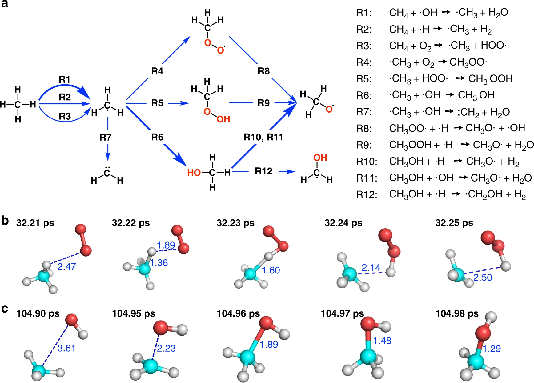The initial stage of combustion

Fig: The initial stage of combustion. The figure is taken from this paper and more results can be found there.

Acknowledge

This work was supported by the National Natural Science Foundation of China (Grants No. 22173032, 21933010). J.Z. was supported in part by the National Institutes of Health (GM107485) under the direction of Darrin M. York. We also thank the ECNU Multifunctional Platform for Innovation (No. 001) and the Extreme Science and Engineering Discovery Environment (XSEDE), which is supported by National Science Foundation Grant ACI-1548562.56 (specifically, the resources EXPANSE at SDSC through allocation TG-CHE190067), for providing supercomputer time.

References

Jinzhe Zeng, Liqun Cao, Tong Zhu (2022), Neural network potentials, Pavlo O. Dral (Eds.), Quantum Chemistry in the Age of Machine Learning, Elsevier.
Jinzhe Zeng, Liqun Cao, Mingyuan Xu, Tong Zhu, John Z. H. Zhang, Complex reaction processes in combustion unraveled by neural network-based molecular dynamics simulation, Nature Communications, 2020, 11, 5713.
Frisch, M.; Trucks, G.; Schlegel, H.; Scuseria, G.; Robb, M.; Cheeseman, J.; Scalmani, G.; Barone, V.; Petersson, G.; Nakatsuji, H., Gaussian 16, revision A. 03. Gaussian Inc., Wallingford CT 2016.
Han Wang, Linfeng Zhang, Jiequn Han, Weinan E, DeePMD-kit: A deep learning package for many-body potential energy representation and molecular dynamics, Computer Physics Communications, 2018, 228, 178-184.
Aidan P. Thompson, H. Metin Aktulga, Richard Berger, Dan S. Bolintineanu, W. Michael Brown, Paul S. Crozier, Pieter J. in ‘t Veld, Axel Kohlmeyer, Stan G. Moore, Trung Dac Nguyen, Ray Shan, Mark J. Stevens, Julien Tranchida, Christian Trott, Steven J. Plimpton, LAMMPS - a flexible simulation tool for particle-based materials modeling at the atomic, meso, and continuum scales, Computer Physics Communications, 2022, 271, 108171.
Denghui Lu, Wanrun Jiang, Yixiao Chen, Linfeng Zhang, Weile Jia, Han Wang, Mohan Chen, DP Train, then DP Compress: Model Compression in Deep Potential Molecular Dynamics, 2021.
Jinzhe Zeng, Liqun Cao, Chih-Hao Chin, Haisheng Ren, John Z. H. Zhang, Tong Zhu, ReacNetGenerator: an automatic reaction network generator for reactive molecular dynamics simulations, Phys. Chem. Chem. Phys., 2020, 22 (2), 683–691.

Learning Resources

Here is the learning Resources:

Video Tutorials（Chinese)

Some Video Resources：

Basic theoretical courses:

DeePMD-kit and DP-GEN

Writing Tips

Hello volunteers, this docs tells you how to write articles for DeepModeling tutorials.

You can just follow 2 steps:

Write in markdown format and put it into proper directories.
Change index.rst to show your doc.

Write in Markdown and Put into proper directories.

You should learn how to write a markdown document. It is quite easy!

Here we recommend you 2 website:

You should know the proper directories.

Our Github Address is: https://github.com/deepmodeling/tutorials

All doc is in: “source” directories. According to your doc’s purpose, your doc can be put into 4 directories in “source”:

Tutorials: Telling beginners how to run Deepmodeling projects.
Casestudies: Some case telling people how to use Deepmodeling projects.
Resources: Other resources for learning.
QA: Some questions and answers.

After that, you should find the proper directories and put your docs.

For example, if you write a “methane.md” for case study, you can put it into “/source/CaseStudies/Gas-phase”.

Change indexs.rst to show your doc.

Then you should change the index.rst to show your doc.

You can learn rst format here: reStructuredText

In short, you can simply change index.rst in your parent directories.

For example, if you put “methane.md” into “/source/CaseStudies/Gas-phase”, you can find and change “index.rst” in “source/CaseStudies/Gas-phase”. All you should do is imitating such file. I believe you can do it!

If you want to learn more detailed information about how to build this website, you can check this:

Q & A

here is Q & A

讨论和反馈:

这些教程需要你的反馈。如果你认为有些教程是混乱的，请在我们的`讨论板<https://github.com/deepmodeling/tutorials/discussions>`上写下你的反馈意见。

目前的工作:

目前，我们正在为以下项目编写教程:

DeePMD-Kit
DP-GEN

另一个团队正专注于为初学者编写一些AI + Science的简要材料，如。

什么是机器学习
什么是分子动力学模拟
关于AI + Science的核心概念